Integration of area detector data in GSAS-II
In this demo, data collected with a Perkin-Elmer area detector at APS 11-ID-C with a wavelength 0.10798 A, where the detector was intentionally tilted at 45 degrees, are used. Note that menu entries are listed in bold face below as Help/About GSAS-II, which lists first the name of the menu (here Help) and second the name of the entry in the menu (here About GSAS-II).
Prerequisite: Calibration Demo
This assumes that an image data set has been read in and calibration results have been derived, see Calibration of an area detector in GSAS.
Step 1: Clear calibration plot
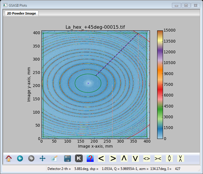
Assuming the previous step was calibration, the image plot will show the located rings and possibly all the picked points. These are no longer needed. Go to the Image Controls window on the data tree. The Calibration/Clear Calibration menu entry removes these from the plot, but does not clear the calibration results. Use of this menu item is not required, but does speed future display of results.
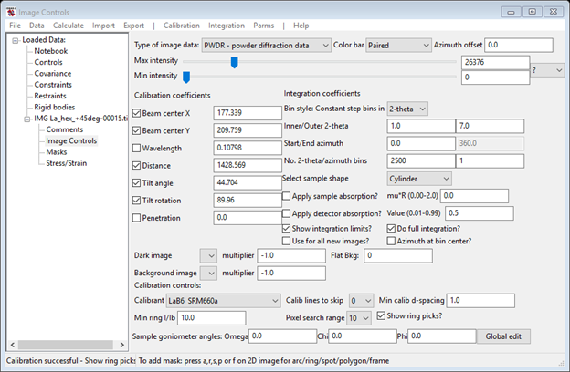
Step 2: Integration Settings
In the simplest case, all that is needed is to click on the Do full integration? check box and adjust the inner and outer 2-theta values with the Inner 2-theta and Outer 2-theta controls. It is helpful to see the two-theta limits on the plot visually, while adjusting the two-theta range. This is done by clicking on the Show integration limits? check box (if not already checked). Note that inner limit is shown as a green ellipse at 2deg and the outer is shown as a red ellipse at 5deg by default. These limits may also be dragged to the desired values; a small popup window shows the value.
Change the limits to 1 and 7 for this data. Note that changes are displayed when numbers are placed in the boxes only after pressing return or tab key or by clicking on some other item in the window.
Other useful controls:
Azimuth offset: The image horizontal axis (from the beam center, going right) is labeled with the azimuth value placed in the Azimuth offset box. This is usually zero unless the image plate has been rotated about its normal axis.
Start/End azimuth: The integration is started at the Start azimuth angle in the left box, and when the Do full integration? check box is not checked, the integration will be run only to the maximum value specified. When the range is less than 360 degrees, the integration range will be shown (if selected) with the high and low limits plotted and only segments of the max and min ellipses drawn. These limits may also be dragged on the plot to desired locations. In this case 45 is a better choice than the default.
Number of 2-theta bins: The resulting 1-D powder pattern after integration will consist of this many points. This number should be on the order of the number of pixels in one direction (since resolution cannot be much better than this) or less, if instrumental resolution and sample broadening does not require that many points. Some trial and error may be needed, but there should more than 6 points across each peak full-width-at-half-maximum (FWHM) in the final pattern to be useful for further analysis. For this reason 5000 is a better choice than the default in that first box.
Number of azimuth bins: In cases where the diffraction experiment shows changes as a function of azimuthal angle, the integration can be performed as a function of angle. This number specifies the number of bins to use by azimuthal angle. The process of breaking up the integration in this way is sometimes called "caking" since the integration region grows with distance from the beam-center, with a shape like a slice of cake or pie. When more than one azimuthal bin is used, the regions are shown in the plot with dashed lines, when the Show integration limits? check box, if not already checked.
Apply Sample absorption and value: An absorption correction for a horizontal cylinder is applied to the results of the integration. The range in mR is limited because the correction is unreliable for mR > 2.
Apply detector absorption and value: The scattered ray beams are partially absorbed by the detector depending on the scattering angle. This reduces the intensity of higher angle data more than low angle data. The value is dependent on the wavelength and the materials used for the front surface of the detector, so some experimentation with a standard is needed to establish an appropriate value.
Dark image and Multiplier: You can designate a previously read in dark image (if the image acquisition software hasn’t already subtracted it!); it will immediately be applied to the visible image so you will see the result of the removal of the dark image. Note that the Multiplier must be negative for it to be subtracted. Note that all images used in this way must be exactly the same format (number of pixels & pixel size).
Background image and Multiplier: You can designate a previously read in image as background which will then be used to modify each data image as they are integrated. Note that the Multiplier must be negative for it to be subtracted. Note that all images used in this way must be exactly the same format (number of pixels & pixel size).
Flat Bkg: Instead of subtracting a background image (you might not have one!), you can subtract a constant. Use the cursor to find a reasonable value to enter here; it is immediately applied to the image.
Step 3: Perform integration
Use the Integration/Integrate image data menu item to start the integration. This will take at least a few seconds. If multiple images have been read in, the Integrate All menu item can be used. This is most useful when the Use as Default option is in use for one image.
At this point the data tree window will have new entries as each azimuthal "slice" added to the data tree as a powder pattern

A plot is added to the plot window with a conventional 1-D powder pattern(s) for each "slice"

Again you could save the project with File/Save project on the main GSAS-II data tree menu although it is not needed for any further tutorials.